Introducció a mapes amb R
Lluís Ramon
22 de abril de 2014
Objectius
- Entendre estructura dades espacials
- Tractar dades espacials amb R
- Conèixer packages per representar mapes
- Crear mapes temàtics
- Crear mapes sobre Google Maps
- Crear mapes dinàmics
Tipus objectes espacials
- Points (escoles, empreses alimentaries, …)
- Lines (carreteres, rius, …)
- Polygons (paisos, comarques, …)
- Grid/Raster (informació per cada cel·les)
Només tractarem Points i Polygons
- Polygons: Mapes temàtics
- Points: Mapes sobre Google Maps
Importarem informació Polygons d’un shapefile.
Es podria crear amb R però complicat Spatial Cheatsheet.
Què és un Shapefile?
Format intercanvi informació geogràfica.
- shp: emmagatzema entitats geomètriques dels objectes
- dbf: emmagatzema informació dels atributs dels objectes
- shx: emmagatzema l’índex de les entitats geomètriques
Molts organismes oficials ofereixen les dades geogràfiques en aquest format.
Importar mapa d’europa
- getinfo.shape
- readShapeXXX
(XXX: Spatial, Points, Lines, Poly)
library(maptools)
getinfo.shape("data/europa.shp")
## Shapefile type: Polygon, (5), # of Shapes: 32
europa <- readShapePoly("data/europa.shp")
Què és europa? Un list? Un data.frame?
Estructura dades espacials
Llibreria sp
- Objectes: Conté atributs que descriuen l’objecte
- Mètodes: Funcions sobre els objectes
- Benficis com: Inheritance, Polymorphism, Encapsulation, etc.
Estructura sp
is(europa)
## [1] "SpatialPolygonsDataFrame" "SpatialPolygons"
## [3] "Spatial"
isS4(europa)
## [1] TRUE
getClass("SpatialPolygonsDataFrame")
## Class "SpatialPolygonsDataFrame" [package "sp"]
##
## Slots:
##
## Name:         data    polygons   plotOrder        bbox proj4string
## Class:  data.frame        list     integer      matrix         CRS
##
## Extends:
## Class "SpatialPolygons", directly
## Class "Spatial", by class "SpatialPolygons", distance 2
slotNames(europa)
## [1] "data" "polygons" "plotOrder" "bbox" "proj4string"
str(europa, max.level = 2)
## Formal class 'SpatialPolygonsDataFrame' [package "sp"] with 5 slots
##   ..@ data       :'data.frame':  32 obs. of  5 variables:
##   .. ..- attr(*, "data_types")= chr [1:5] "C" "N" "C" "N" ...
##   ..@ polygons   :List of 32
##   ..@ plotOrder  : int [1:32] 31 28 13 12 24 11 7 25 32 17 ...
##   ..@ bbox       : num [1:2, 1:2] -10.5 34.6 44.8 71.2
##   .. ..- attr(*, "dimnames")=List of 2
##   ..@ proj4string:Formal class 'CRS' [package "sp"] with 1 slots
bbox(europa)
##      min   max
## x -10.48 44.82
## y  34.57 71.17
names(europa)
## [1] "SP_ID" "STAT_LEVL_" "NUTS_ID" "SHAPE_Leng" "SHAPE_Area"
summary(europa)
## Object of class SpatialPolygonsDataFrame
## Coordinates:
##      min   max
## x -10.48 44.82
## y  34.57 71.17
## Is projected: NA
## proj4string : [NA]
## Data attributes:
##      SP_ID      STAT_LEVL_    NUTS_ID     SHAPE_Leng      SHAPE_Area
##  AT     : 1   Min.   :0    AT     : 1   Min.   :  2.9   Min.   : 0.33
##  BE     : 1   1st Qu.:0    BE     : 1   1st Qu.: 18.5   1st Qu.: 5.73
##  BG     : 1   Median :0    BG     : 1   Median : 29.5   Median : 9.75
##  CH     : 1   Mean   :0    CH     : 1   Mean   : 59.1   Mean   :22.89
##  CY     : 1   3rd Qu.:0    CY     : 1   3rd Qu.: 70.9   3rd Qu.:35.53
##  CZ     : 1   Max.   :0    CZ     : 1   Max.   :451.6   Max.   :81.24
##  (Other):26                (Other):26
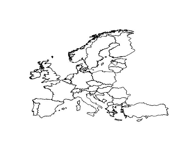
Gràfic base
plot(europa)
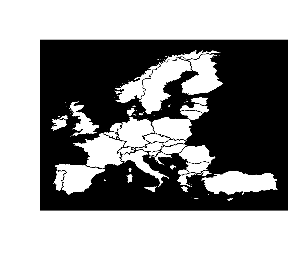
plot(europa, bg = "black", col = "white")
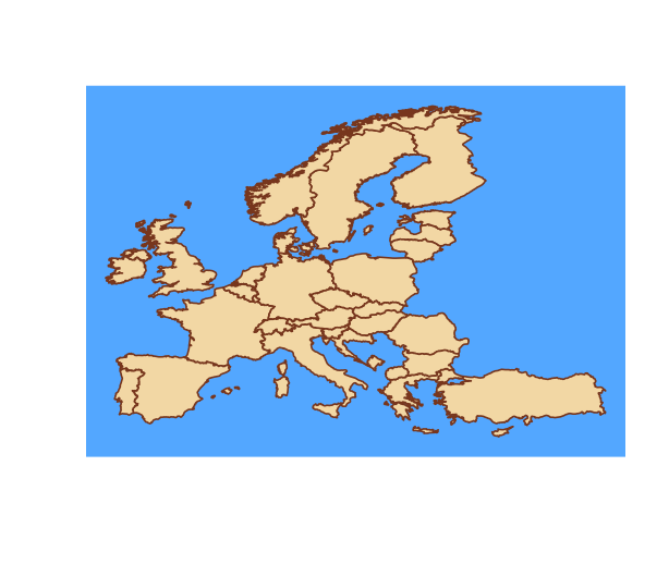
plot(europa, bg = "steelblue1", col = "wheat", border = "sienna4", lwd = 1.6)
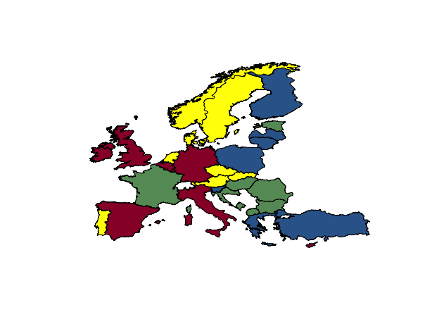
Preus europeus de l’electricitat
Continuació entrada Evolució del preu de l’electricitat
load("data/preu_elec.RData")
head(preu_elec)
##   geo  a2004  a2007  a2010  a2013 col2013
## 3  AT 0.0981 0.1050 0.1427 0.1413 #FFFF00
## 5  BE 0.1145 0.1229 0.1449 0.1583 #990033
## 6  BG 0.0486 0.0547 0.0675 0.0771 #669966
## 7  CY 0.0928 0.1177 0.1597 0.2277 #990033
## 8  CZ 0.0660 0.0898 0.1108 0.1249 #FFFF00
## 9  DE 0.1259 0.1433 0.1381 0.1493 #990033
Creuar dades europa
merge accepta un Spatial i un data.frame.
europa_elec <- merge(europa, preu_elec, by.x = "SP_ID", by.y = "geo")
is(europa_elec)
## [1] "SpatialPolygonsDataFrame" "SpatialPolygons"
## [3] "Spatial"
head(europa_elec@data)
##   SP_ID STAT_LEVL_ NUTS_ID SHAPE_Leng SHAPE_Area  a2004  a2007  a2010
## 0    AT          0      AT     24.860    10.0283 0.0981 0.1050 0.1427
## 1    BE          0      BE     14.006     3.8969 0.1145 0.1229 0.1449
## 2    BG          0      BG     21.372    12.2090 0.0486 0.0547 0.0675
## 3    CH          0      CH     17.455     4.8663     NA     NA     NA
## 4    CY          0      CY      6.326     0.9189 0.0928 0.1177 0.1597
## 5    CZ          0      CZ     20.822     9.8424 0.0660 0.0898 0.1108
##    a2013 col2013
## 0 0.1413 #FFFF00
## 1 0.1583 #990033
## 2 0.0771 #669966
## 3     NA    <NA>
## 4 0.2277 #990033
## 5 0.1249 #FFFF00
col a vector of colour values
plot(europa_elec, col = europa_elec$col2013)
spplot
colors <- colorRampPalette(c("#669966", "#336699", "#FFFF00", "#990033"))(32)
spplot(europa_elec, zcol = c("a2010", "a2013", "a2004", "a2007"), col.regions = colors)
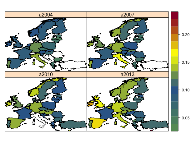
- Paleta de colors sobre tots els anys
- Utilitza package lattice. Funcionament semblant.
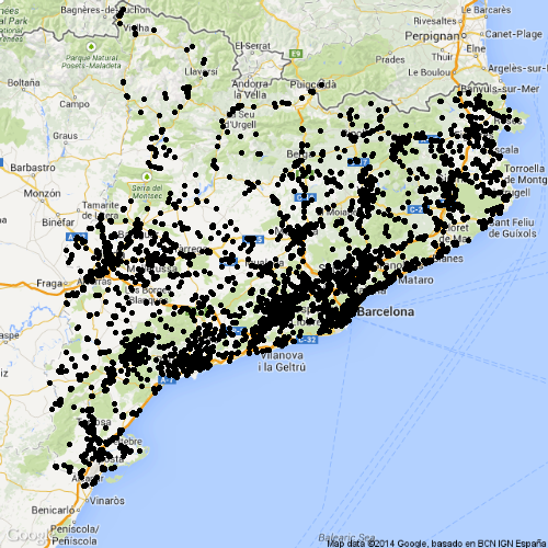
Mapa de industries agraries i alimentaries de Catalunya
Dades del Registre d’indústries agràries i alimentàries de Catalunya (RIAAC).
load("data/ind_ali.RData")
head(ind_ali)
##                             establiment             sector      x       y
## 1                   A. I J. GARGANTA SL Alimentació animal 510067 4654945
## 2             ABONOS ORGANICOS BOIX, SL    Altres agràries 445675 4645225
## 3                   ABSOLUTUS OLEUM, SL     Olis i greixos 302692 4546957
## 4    ACABADOS DOUBLE FACE DEL VALLES SA    Altres agràries 440397 4609387
## 5 ACABADOS ESPECIALES VIC SA (AESVICSA)    Altres agràries 440348 4644908
## 6                     ACCES FILTERS, SL          Forestals 462962 4623129
- He simplificat i reduït els camps.
- Coordenades en UTM.
- Farem un mapa amb fons de Google Maps. Requereix coordenades LonLat.
Canviar sistema de coordenades
Llibreria rgdal
Funció spTransform, CRS
library(rgdal)

coord_utm <- CRS("+proj=utm +zone=31")
coord_LonLat <- CRS("+proj=longlat")

ind_sp_utm <- SpatialPoints(ind_ali[, c("x", "y")], proj4string = coord_utm)
ind_sp_LonLat <- spTransform(ind_sp_utm, coord_LonLat)
lon <- coordinates(ind_sp_LonLat)[, 1]
lat <- coordinates(ind_sp_LonLat)[, 2]
ind_ali_LonLat <- cbind(ind_ali[, c("establiment", "sector")], lon, lat)

head(ind_ali_LonLat)
##                             establiment             sector    lon   lat
## 1                   A. I J. GARGANTA SL Alimentació animal 3.1216 42.05
## 2             ABONOS ORGANICOS BOIX, SL    Altres agràries 2.3445 41.96
## 3                   ABSOLUTUS OLEUM, SL     Olis i greixos 0.6522 41.05
## 4    ACABADOS DOUBLE FACE DEL VALLES SA    Altres agràries 2.2844 41.63
## 5 ACABADOS ESPECIALES VIC SA (AESVICSA)    Altres agràries 2.2802 41.95
## 6                     ACCES FILTERS, SL          Forestals 2.5545 41.76
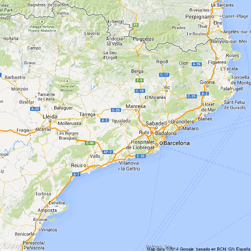
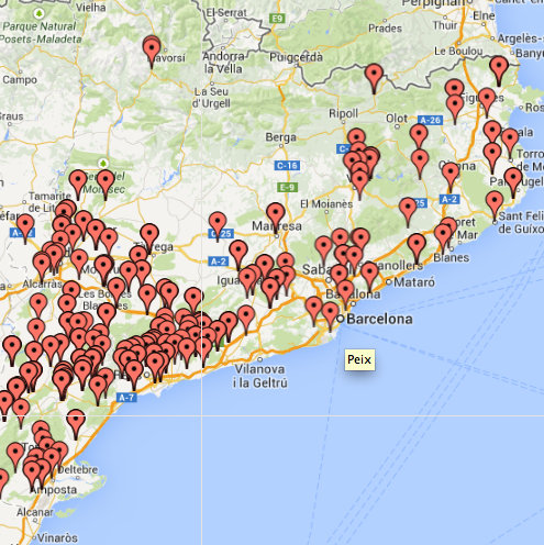
RGoogleMaps
library(RgoogleMaps)
mapa_fons <- GetMap.bbox(ind_ali_LonLat$lon, ind_ali_LonLat$lat)
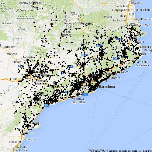
PlotOnStaticMap(mapa_fons)

PlotOnStaticMap(mapa_fons, ind_ali_LonLat$lat, ind_ali_LonLat$lon, pch = 19, cex = 0.7)
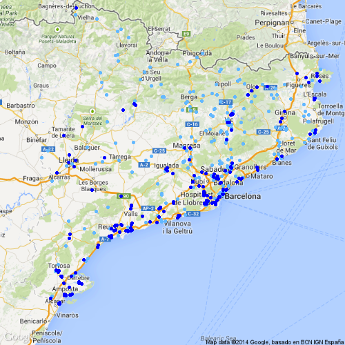
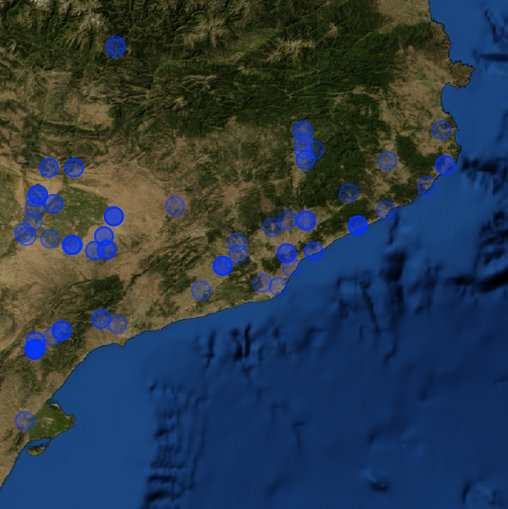
cond <- ind_ali_LonLat$sector == "Lactis"
ind_lac <- ind_ali_LonLat[cond, ]

cond <- ind_ali_LonLat$sector == "Peix"
ind_peix <- ind_ali_LonLat[cond, ]

PlotOnStaticMap(mapa_fons, ind_lac$lat, ind_lac$lon, pch = 19, cex = 0.7, col = "steelblue1")
PlotOnStaticMap(mapa_fons, ind_peix$lat, ind_peix$lon, pch = 19, cex = 0.7, col = "blue", add = TRUE)
ggplot2 + ggmap
library(ggmap)
center = c(mean(ind_ali_LonLat$lon), mean(ind_ali_LonLat$lat))
zoom <- min(MaxZoom(range(ind_ali_LonLat$lat), range(ind_ali_LonLat$lon))) # MaxZoom es de RgoogleMaps
mapa <- get_map(location = center, zoom = zoom, maptype =  "roadmap")
ggmap(mapa, extent = "device")
ggmap(mapa, extent = "device") + geom_point(data = ind_ali_LonLat, aes(lon, lat))
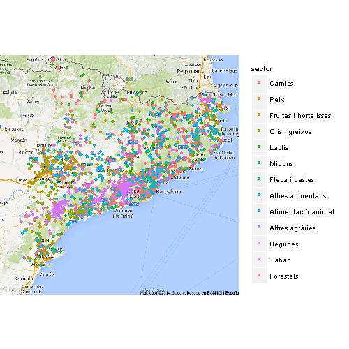
ggmap(mapa, extent = "device") +
  geom_point(data = ind_ali_LonLat, aes(lon, lat, colour = sector))
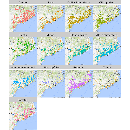
ggmap(mapa, extent = "device") +
  geom_point(data = ind_ali_LonLat, aes(lon, lat, colour = sector), size = 0.8) +
  facet_wrap(~sector) + guides(colour = FALSE)
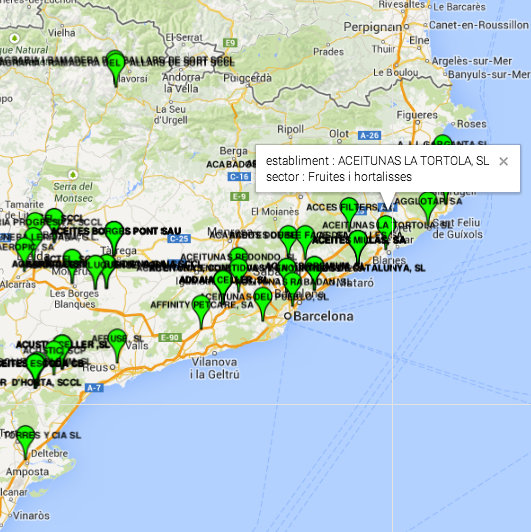
plotGoogleMaps
library("plotGoogleMaps")
ind_sp <- SpatialPointsDataFrame(ind_sp_LonLat, ind_ali[, c("establiment", "sector")])
plotGoogleMaps(ind_sp[1:99, ], filename = "Mapes dinamics/plotGoogleMaps.html", mapTypeId = "ROADMAP")
LeafletR
library("leafletR")
leaflet <- toGeoJSON(data = ind_ali_LonLat[1:99, c("lat",  "lon", "sector")], dest = "Mapes dinamics", name = "leaflet")
ind_html <- leaflet(data = leaflet, dest = "leaflet", popup ="sector", base.map="mqsat", incl.data = TRUE)
browseURL(ind_html)
googleVis
library(googleVis)
ind_ali_LonLat$LatLong <- paste(ind_ali_LonLat$lat, ind_ali_LonLat$lon, sep = ":")
indGoogleVis <- gvisMap(ind_ali_LonLat, "LatLong",
                        options = list(useMapTypeControl = TRUE,
                                       width = 800,height = 800))
print(indGoogleVis, file = "Mapes dinamics/googleVis.html")
Quins packages NO hem usat?